Traditionally, sequence reads are clustered into operational taxonomic units (OTUs) at a defined identity threshold to avoid sequencing errors generating spurious taxonomic units. However, with the bioinformatic technique advancement, recently several bioinformatic software can correct sequencing errors to determine real biological sequences at single nucleotide resolution by generating amplicon sequence variants (ASVs) or sub-OTUs. Both ASVs and sub-OTUs are 100% OTUs and supposedly have 100% identities to clinical variation. The two most widely used denoising packages DADA2 (Callahan et al. 2016b) and Deblur (Amir et al. 2017) have been warped into QIIME 2. In this chapter, we describe and illustrate their uses to generate ASVs or sub-OTUs. First, we introduce how to analyze the demultiplexed paired-end FASTQ data (Sect. 4.1), and then we introduce DADA2 and q2-dada2 plugin and how to use them to analyze demultiplexed paired-end FASTQ data (Sect. 4.2) and analyze the multiplexed paired-end FASTQ data using q2-dada2 plugin (Sect. 4.3), respectively. Next, we introduce Deblur and q2-deblur plugin and how to use them to analyze demultiplexed paired-end FASTQ data (Sect. 4.4). Finally, we briefly summarize in this chapter (Sect. 4.5).
4.1 Analyzing Demultiplexed Paired-End FASTQ Data
The sample paired-end fastq data and metadata we analyze here are from a published paper by Schloss et al. (2012) entitled “Stabilization of the murine gut microbiome following weaning.” We have introduced this data in Example 3.9. Here and in other chapters of this book, we use this dataset to illustrate bioinformatic analysis using QIIME 2 and statistical analysis using R. We downloaded the data from http://www.mothur.org/MiSeqDevelopmentData/StabilityNoMetaG.tar. You can download, unzip, and save this dataset into the directory on your computer, and then you can use the following R function list.files() or software seqkit to open the raw sequence data.
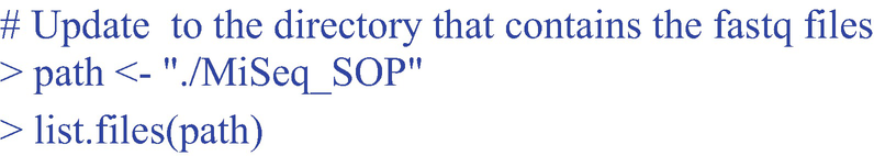
A raw sequence data in 3 rows. 1. Hashtag update to the directory that contains the fast q files. 2. Greater than path less than negative double quotation dot forward slash M i S e q underscore S O P double quotation. 3. Greater than list dot files, open bracket, path, closed bracket.
Here we extract some rows of them below to give you some idea of these raw sequence data.
A raw sequence of data in 12 rows.
4.1.1 Prepare Sample Metadata
Sample metadata contains important biological information in microbiome analysis. They are created typically to collect data information on technical details (i.e., the DNA barcodes), descriptions of the experiment design and samples (i.e., the group, subject, time point, and body site that the sample belongs to). There are no specific restrictions on what types of sample metadata should be used and no enforced “metadata standards” in QIIME 2; however, QIIME 2 does provide some general formatting requirements when creating metadata. For example, although data with any file extensions can be used in QIIME 2, QIIME 2 prefers that sample metadata is stored in a tab-separated values (TSV) file rather than other formats such as the common used comma-separated values (CSV) format. The reason that QIIME 2 uses TSV instead of CSV is that CSV needs to use escape commas which often causes difficulties.
Identifier Column. The identifier (ID) column is the first column in the metadata file, which defines the sample IDs for sample metadata. The ID column name (i.e., ID header) must be one of the following case-insensitive values, and they are not allowed to be used for naming other IDs or columns in the file: id, sampleid, sample id, sample-id, featureid, feature id, and feature-id.
IDs. IDs may consist of any unicode characters excepting starting with the pound sign (#). One file needs at least one ID. IDs must be unique, but cannot be empty, and cannot use any of the reserved ID column names listed above.
Identifiers. Identifiers should be less or equal to 36 characters, and contain only ASCII alphanumeric characters (i.e., in the range of [a-z], [A-Z], or [0-9]), the period (.) character, or the dash (-) character.
Column Types. QIIME 2 currently supports both categorical and numeric metadata columns. By default, if one column consists only of numbers or missing data, then QIIME 2 will treat the type of metadata column as numeric. Otherwise, if the column contains any non-numeric values, QIIME 2 will treat the column as categorical. Both categorical columns and numeric columns support missing data (i.e., empty cells).
Step 1: Collect the study design and sample information using an Excel sheet.
Step 2: Upload the Excel sheet into Google sheet.
First go to Google Drive homepage and log in using your credentials. In the Google Drive homepage, click New ➔ select Google Sheets➔click File➔Import➔in Import file screen, click Upload➔ then you can either drag the SampleMetadata excel sheet file to the box, or click Select a file from your device➔then open the file. In the Import file screen, default option is “Replace spreadsheet”; just choose it and click Import data. Then the SampleMetadata.xlsx was uploaded into Google Sheet.
Step 3: Install open source Google sheets add-on Keemei program.
QIIME 2 needs sample metadata spreadsheet correctly formatted. You can set this file as a Google sheet and then use the Keemei (canonically pronounced key may) program (Rideout et al. 2016) for Google sheets to check whether the file is correctly formatted. Keemei is an open source Google Sheets add-on for cloud-based validating tabular bioinformatics file formats, including QIIME 2 metadata files. To install Keemei, first log in to your free Google account, then you have two options to install Keemei to your Google sheets. (1) Go to https://keemei.qiime2.org/ webpage, click the Chrome Web Store, and then click INSTALL and follow the direction to install. (2) From within a Google Sheet: click and search for Keemei. Once Keemei is installed, you can use it to validate the SampleMetadata.xlsx file.
Step 4: Check whether the sample metadata spreadsheet is correctly formatted using Keemeil.
To validate the SampleMetadata.xlsx, click File➔Make a copy, and name it as Copy of SampleMetadata. Now you can start to validate the sample metadata with Keemei. To validate this active sheet, click Add-ons➔Validate QIIME 2 metadata file. When you see Keemeil validation report says “Good news! Sheet metadata is a valid QIIME 2 metadata file,” then your spreadsheet is correctly formatted for QIIME 2. In this case, the SampleMetadata spreadsheet passes Keemei validation. Now, click File again and choose Download as Table-separated values (.tsv, current sheet). You now can save and rename it as what you want. In this case, we name it as SampleMetadataMiSeq_SOP.tsv.
Once this spreadsheet is correctly formatted for QIIME 2, the file is ready for use. If cells come out with red, it suggests that these cells have errors; if cells come out with yellow, which suggests that these cells have warnings. Then a sidebar summaries the validation report and lists invalid cells. Locate the cells with errors and warnings, fix all the invalid cells, and revalidate until all cells are valid. To clear the validation status on the active sheet, by clicking Add-ons➔Keemei➔Clear validation status, the cell background colors will reset to white and notes will be cleared.
Step 5: Further inspect the sample metadata in QIIME 2.
To further inspect the sample metadata in QIIME 2, create a working directory (here, QIIME2R-Bioinformatics) and put the SampleMetadataMiSeq_SOP.tsv in this working directory.
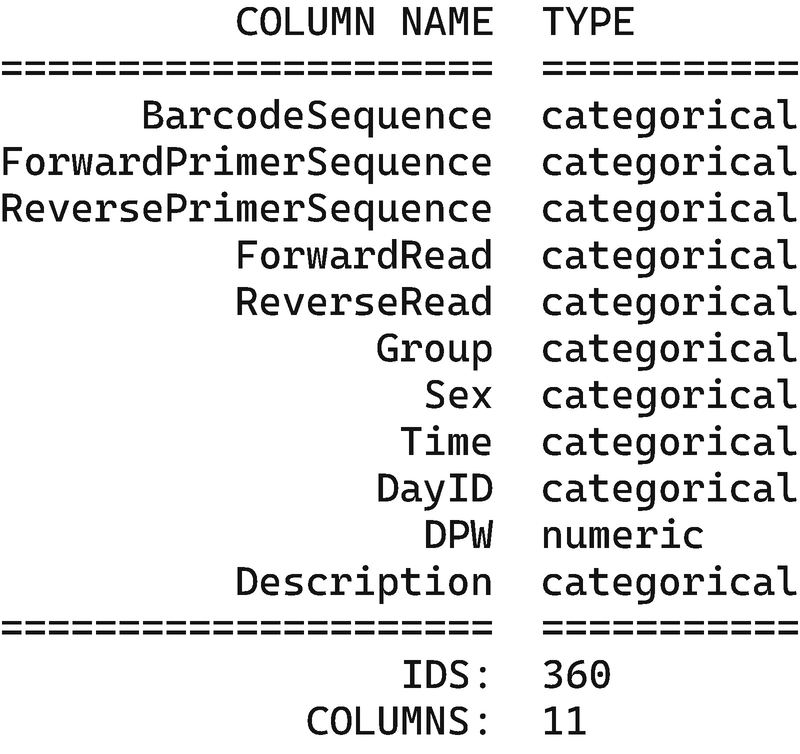
A table of two columns titled column name and type. The column names are barcode sequence, forward and reverse primer sequences, forward read, reverse read, group, sex, time, day I D, D P W, and description. The I D S is 360, and the Columns are 11.
Inspection of sample metadata for the mouse gut microbiome study
4.1.2 Prepare Raw Sequence Data
Different sequencing platforms (e.g., Illumina vs. Ion Torrent) or different sequencing approaches (e.g., single-end vs. paired-end) will provide us different structured raw data. In addition, any pre-processing steps such as joined paired ends and barcodes in fastq header performed by sequencing centers also will result in different structured raw data.
Now the files are ready for analysis. Currently two approaches are available in QIIME 2 to construct a feature table from raw reads: either using data2 or deblur plugins. We illustrate their uses respectively as below.
4.1.3 Import Data Files as Qiime Zipped Artifacts(.qza)
QIIME 2 works with artifacts (.qza). We must first import the FASTQ files as a QIIME artifact using the import command qiime tools import. As we described in Chap. 3, if the data do not have either EMP or Casava format, the data need to be manually imported into QIIME 2. First you need to create a tab-separated (i.e., .tsv) “manifest” text file. In this case, we created a manifest file called ManifestMiSeq_SOP.tsv as the same way we created the SampleMetadataMiSeq_SOP.tsv and stored it in the same working directory: QIIME2R-Bioinformatics.

A text reads, imported manifest M i S e q underscore S O P dot t s v as Paired End fast q manifest P h r e d 33 V 2 to Paired End demux M i S e q underscore S O P dot q z a.
QIIME 2 uses SampleData[PairedEndSequencesWithQuality] to indicate the sequence data for each sample are paired forward/reverse FASTQ files. So we specify the data type as 'SampleData[PairedEndSequencesWithQuality]'. We specify input data format as PairedEndFastqManifestPhred33V2 and name the output artifact as PairedEndDemuxMiSeq_SOP.qza. This file will contain a copy of each of the sequence data files, which will enhance research reproducibility.
You can check this qiime zipped artifact (.qza) using qiime tools peek command.
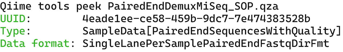
A 4-line text. The title is Qiime tools peek Paired End Demux M i S e q underscore S O P dot q z a. It presents details about U U I D, type, and data format.
4.1.4 Examine and Visualize the Qualities of the Sequence Reads
To generate visualizations of the sequence qualities, you can run the command:

A text reads, saved visualization to, Paired End Demux M i S e q underscore S O P dot q z v.

A text reads, saved visualization to, Paired End Demux M i S e q underscore S O P dot q z v.
To review the visualization of the PairedEndDemuxMiSeq_SOP.qzv file, you can navigate to QIIME2 viewer in browser. In other words, copy over the PairedEndDemuxMiSeq_SOP.qzv output to your computer, and open this file in www.view.qiime2.org. The following plot is from the interactive quality plot.
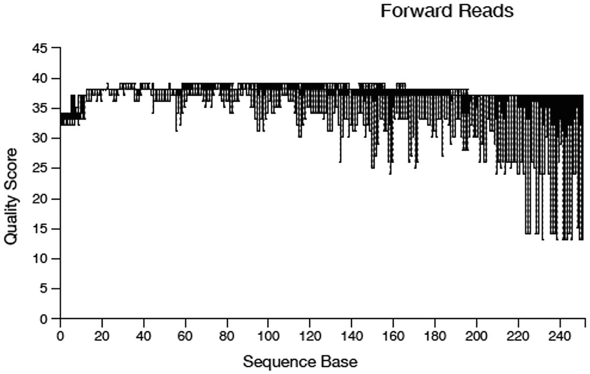
A boxplot of quality score versus sequence base. The title is forward reads. It displays a decreasing trend. The quality score for the forward reads range from 15 to 40. The values are approximated.
Quality score box plots sampled from 10,000 random forward reads
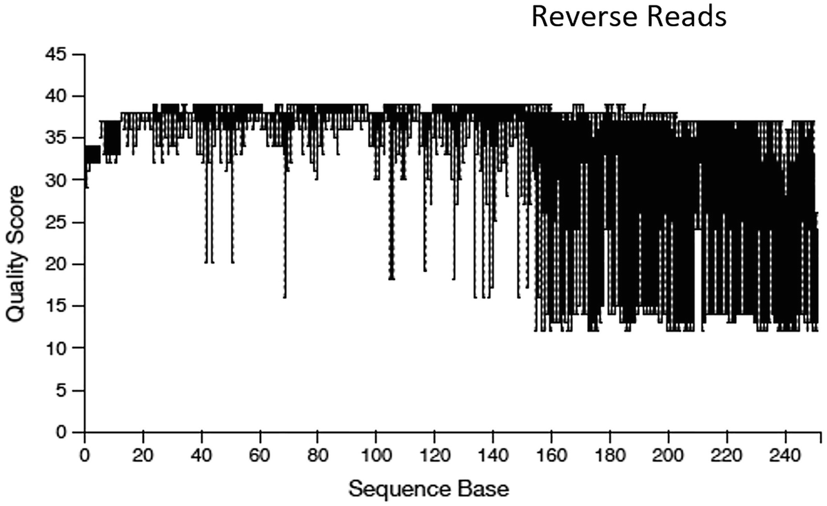
A boxplot of quality score versus sequence base. The title is reverse reads. It displays a decreasing trend. The quality score for the reverse reads range from 10 to 40. The values are approximated.
Quality score box plots sampled from 10,000 random reverse reads
Illumina sequencing data generally show a trend of decreasing average quality towards the end of sequencing reads. In this case, the forward reads and the reverse reads display different patterns of quality: the forward reads maintain high quality over through, whereas the quality of the reverse reads drops significantly at around the position 160. Based on the different quality information for forward and reverse reads, we differentially truncate the forward reads at position 240, and the reverse reads at position 160 as did by Callahan et al. (2016a).
We also notice that both quality plots have slightly lower quality scores at the beginning of each read, which are caused by the homogeneity of the primer sequences. It is difficult for Illumina sequencer to properly identify clusters of DNA molecules (Fadrosh et al. 2014). Thus, the primer sequences must be removed at the denoising stage. Typically, the first 10 nucleotides of each read will be trimmed based on empirical observations across many Illumina datasets because these base positions are particularly likely to contain pathological errors (Callahan et al. 2016a).
4.2 Analyzing Demultiplexed Paired-End FASTQ Data Using DADA2 and q2-dada2 Plugin
The 16S rRNA marker gene sequencing approach has several advantages (Xia et al. 2018) including its own unique structure that contains both conserved and variable regions and its presence in all known Bacteria and Archaea species. This sequencing approach also has the advantages compared to shotgun metagenomic sequencing: low cost and avoid of problems with sequencing non-microbial DNA from host contamination. However, the 16S rRNA marker gene sequencing approach has the issue of sequencing errors, which makes it difficult to distinguish biologically real nucleotide differences in 16S sequences from sequencing artifacts. For example, traditionally the OTU method clusters sequence reads into Operational Taxonomic Units (OTUs). This method is used by most of the available pipelines (Caporaso et al. 2010; Schloss 2020; Mysara et al. 2017; Kumar et al. 2011; Hildebrand et al. 2014). However, the OTU method has several fundamental weaknesses such as clustering sequences with a fixed 3% dissimilarity threshold might avoid fine-scale variation among sequences (Rosen et al. 2012); therefore it often eliminates biological information present in the data. OTUs are not species; thus their construction is not necessitated by amplicon errors (Callahan et al. 2016a). In Chap. 6, we illustrate how to cluster OTUs via QIIME 2.
The methods for processing and analysis of 16S marker gene sequencing data continue to improve. DADA2(DADA: Divisive Amplicon Denoising Algorithm) (Callahan et al. 2016b) and Deblur (Amir et al. 2017) methods have been developed and recognized as one major advance towards quality control measures through denoising sequences to better discriminate between true sequence diversity and sequencing errors. Performing quality control of the sequences typically is performed prior to taxonomic classification. The goal is to identify the poor-quality reads and residual contamination in the dataset.
In this chapter, we illustrate how to conduct quality controlling sequences or denoising and QC filtering to generate feature table and feature data.
4.2.1 Introduction to DADA2 and q2-dada2 Plugin
DADA2 was proposed to use “amplicon sequence variants” (ASVs) to replace OTUs as the standard unit of marker-gene analysis and reporting (Callahan et al. 2017). DADA2 uses an error-modeling approach for denoising and clustering amplicons and outputs exact sequence variants (or ASVs). DADA2 aims to overcome the fundamental weaknesses of traditional OTU methods, and to improve the performance of newly proposed bioinformatic sequence denoising approaches including UPARSE, MED, mothur (average linkage), and QIIME (uclust) OTU methods (Callahan et al. 2016a). It was demonstrated that DADA2 methods are more accurate compared to these four methods (Callahan et al. 2016a). It was shown (Callahan et al. 2016b) that DADA2 exactly infers sample sequences and resolves differences of as little as one nucleotide. To model and correct Illumina-sequenced amplicon errors, the software package DADA2 was developed. The R package DADA2 can implement the full amplicon workflow from filtering, dereplication, sample inference, chimera identification to merging the paired-end reads (Callahan et al. 2016a). For the details on algorithm and the development of DADA2, the reader is referred to Sect. 8.3.2.4.
Here, we illustrate how to implement the DADA2 methods via the DADA2 plugin in QIIME 2. The DADA2 plugin has several methods to denoise reads, including (1) denoise paired-end, which requires unmerged, paired-end reads (i.e., both forward and reverse); and (2) denoise single-end, which accepts either single-end or unmerged paired-end data. When the unmerged paired-end data are provided, only the forward reads will be used and the reverse reads will be ignored.
Implementing DADA2 and Deblur methods will generate two QIIME 2 artifacts: a FeatureTable[Frequency] and a FeatureData[Sequence]. The FeatureTable[Frequency] artifact contains counts (frequencies) of each unique sequence in each sample in the dataset, and the FeatureData[Sequence] artifact maps feature identifiers in the FeatureTable to the sequences they represent. In QIIME 1, they were called Biom table and rep_set fasta file, respectively.
DADA2 and Deblur are currently the two denoising methods available in QIIME 2. We apply the DADA2 approach to the mouse gut microbiome data (Example 4.1: MiSeq_SOP).
4.2.2 Denoise Sequences to Construct Feature Table and Feature Data with q2-dada2 Plugin
A feature is a species or an OTU in the context of microbiome sequencing or a gene in the RNA-Seq context. Specially in DADA2 and Deblur, features are ASVs or sub-OTUs, respectively. In QIIME 2, denoising Illumina sequence via DADA2 is an alternative option to OTU clustering as defined sequence-identify cut-off (e.g., 97%). The qiime dada2 denoise-paired method performs merging and denoising paired-end reads to denoise paired-end sequences, dereplicate them, and filter chimeras.
The parameters --p-trim-left-f and --p-trim-left-r (optional) are used to trim the 5′ end of the input sequences, which will be the bases that were sequenced in the first cycles. When primers are present in the input sequence files, DADA2 requires removing the primers from the data to prevent false positive detection of chimeras as result of degeneracy in the primers before denoising DADA2 remove the setted length of the primer sequences. The parameter --p-trim-left-f is used to specify an integer for the position at which forward read sequences should be trimmed due to low quality. Default is 0 for not trimming the forward read sequences. The parameter --p-trim-left-r is used to specify an integer for the position at which reverse read sequences should be trimmed due to low quality. Default is 0.
The parameter --p-trunc-len-f indicates the position at which the forward sequence will be truncated and parameter --p-trunc-len-r indicates the position at which the reverse read will be truncated. They are used to truncate the 3′ end of the of the input sequences, which will be the bases that were sequenced in the last cycles. In above Interactive Quality Plot tab in the visualization of PairedEndDemuxMiSeq_SOP.qzv file that was generated by qiime demux summarize command, there are quality scores for each reads. To determine what values to pass for these two parameters (--p-trunc-len-f and --p-trunc-len-r), you should review the Interactive Quality Plot tab. Specifying 0, no truncation or length filtering will be performed.
The parameter --p-max-ee (--p-max-ee-f and --p-max-ee-r for forward reads and reverse reads, respectively) (optional) controls the maximum number of expected errors in a sequence before it is discarded (default is 2). The default 2 is used to enforce a maximum of 2 expected errors per-read (Edgar and Flyvbjerg 2015), which combines the trimming parameter with standard filtering parameters, and is considered as a better filter than simply averaging quality scores (Edgar and Flyvbjerg 2015). DADA2 trims and filters paired reads jointly, i.e., both reads must pass the filter for the pair to pass.
The parameter --p-truncac-q (optional) is used to truncate the sequence after the first position that has a quality score equal to or less than the provided value (default is 2).
The parameter --p-pooling-method (optional) is used to specify pool samples for denoising. By default, samples are denoised independently (“independent”). If it is specified as (“pseudo”), the pseudo-pooling method is used to approximate pooling of samples.
The parameter --p-chimera-method (optional) is used to specify the method (“none,” “pooled,” “consensus”) to remove chimeras. Specifying “none,” no chimera is removed; specifying “pooled,” all reads are pooled prior to chimera detection, while by default (“consensus”), chimeras are detected in samples individually, and sequences are removed if chimeras are found in a sufficient fraction of samples.
The parameter --p-n-threads (optional) is used to specify the number of threads to use for multithreaded. Processing with 1 as default and 0 for using all available cores.
The parameter --p-n-reads-learn (optional) is used to specify the number of reads to use when training the error model. By default, 1,000,000 is used with smaller numbers for a shorter run time but a less reliable error model.
The reader can refer to the QIIME 2 documentation for other input parameters.
Running external command line application(s). This may print messages to stdout and/or stderr.
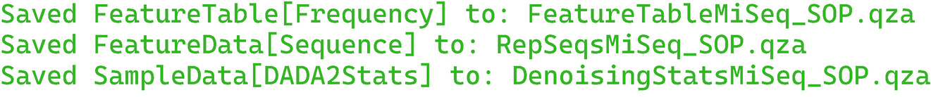
A 3-line text. 1. Saved Feature Table, Frequency, to Feature Table M i S e q underscore S O P dot q z a. 2. Saved Feature Data, Sequence, to R e p S e q s M i S e q underscore S O P dot q z a. 3. Saved Sample Data, D A D A 2 Stats, to Denoising Stats M i S e q underscore S O P dot q z a.
In above commands, we use the parameter --p-n-threads 4 to allow the program to perform parallel computations on 4 threads. If your datasets are very large, DADA2 may be slow. You may need increase the number of threads. The option --verbose is used to display the DADA2 progress in the terminal as shown above. The printed information in the terminal with the --verbose option shows 6 stages of denoising process.
The denoising process outputs three artifacts: (1) a FeatureTable[Frequency] file via --o-table (we named it as FeatureTableMiSeq_SOP.qza), (2) a FeatureData[Sequence] via --o-representative-sequences, which is representative sequence file (we named it as RepSeqsMiSeq_SOP.qza), and (3) an artifact via --o-denoising-stats (DADA 2 Stats , we named it as DenoisingStatsMiSeq_SOP.qza). All these three output file names are required. The feature table file is the Biological Observation Matrix(BIOM) format file. The representative sequence file contains the denoised sequences, while the table file maps each of the sequences onto their denoised parent sequence.
The produced feature table by DADA2 method is a higher-resolution analogue of the common “OTU table”; however, the count reads are called amplicon sequence variants (ASVs) instead of OTUs, which are thought resolving variants that differ by as little as one nucleotide (Callahan et al. 2016b).
4.2.3 Summarize the Feature Table and Feature Data from q2-dada2 Plugin

A text reads, Saved Visualization to, Feature Table M i S e q underscore S O P dot q z v.

A text reads, Saved Visualization to, R e p S e q s M i S e q underscore S O P dot q z v.
The two produced visualization files (.qzv) by the above commands can be explored via the QIIME2 viewer. The “interactive Sample Detail” tab provides detailed information about the denoised sequence counts, such as the number of sequence per sample. We can explore to determine how rarefaction depths (subsampling) will impact your data. For example, we may check which samples have lowest sequencing depths to be dropped.
4.3 Analyzing Multiplexed Paired-End FASTQ Data Using q2-dada2 Plugin
To illustrate the bioinformatic workflow of QIIME 2 and multiplexed paired-end fastq data using QIIME 2, in this section, we demonstrate the steps of analyzing demultiplexed paired-end fastq data using Atacama soil microbiome data.
The data used here was originally from the study of “Significant Impacts of Increasing Aridity on the Arid Soil Microbiome” (Neilson et al. 2017), which analyzes the soil samples from the Atacama Desert in northern Chile. This desert is one of the most arid locations on Earth, where some areas receive less than a millimeter of rain per decade. We downloaded the data from the QIIME 2 website and use the data to illustrate how to denoise sequences to construct a feature table and the associated feature sequences using Deblur along with the importing, demultiplexing, and some other preliminary works.
4.3.1 Prepare Sample Metadata

A text reads, Saved Visualization to, Tabulated Sample Metadata Atacama dot q z v.
4.3.2 Prepare Raw Sequence Data
The paired-end raw sequence data consist of three fastq format files: forward.fastq.gz, reverse.fastq.gz, and barcodes.fastq.gz. They represent forward reads, reverse reads, and barcodes in sequencing run, respectively. Here, we use a 10% subsample data downloaded from QIIME 2 website. We move these three fastq files into the EmpPairedEndSequences working directory we just created and now the files are ready for use. The FASTQ data have the specific format of EMP (EMPPairedEndSequences).
The sequences with the format of EMPPairedEndSequences in QIIME 2 artifacts are multiplexed, suggesting that the sequences have not yet been assigned to samples, and hence to process this kind of sequences, both sequences.fastq.gz and barcodes.fastq.gz files are needed, in which the barcodes.fastq.gz contains the barcode read associated with each sequence in sequences.fastq.gz.
4.3.3 Import Data Files as Qiime Zipped Artifacts(.qza)

A text reads, Imported E m p Paired End Sequences as E M P Paired End D i r F m t to E m p Paired End Sequences Atacama dot q z a.
We can check this qiime zipped artifact (.qza) using qiime tools peek command.
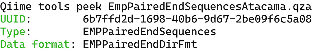
A 4-line text. The topic is Qiime tools peek E m p Paired End Sequences Atacama dot q z a. It provides detail about the U U I D, type, and data format.
4.3.4 Demultiplexing Sequences
The next-generation sequencing instruments are able to analyze multiple samples in a single lane/run through multiplexing these samples. These samples are typically appended a unique barcode (a.k.a. index or tag) sequence to one or both ends of each sequence to identify their originals. Detecting these barcode sequences and mapping them back to the samples they belong to is called demultiplexing sequences.
In QIIME 2, two plugins are available for demultiplexing sequences: q2-demux and q2-cutadapt. However, depending on the type of raw sequence data either EMP Single End, EMP Paired End, Multiplexed Single End Barcode, or Multiplexed Paired End Barcode, usually only one demultiplexing action available in q2-demux or q2-cutadapt for the data. In the case, the barcodes have already been removed from the reads and are in a separate file, then q2-demux can be used; while if the barcodes are still in the sequences, then q2-cutadapt can be used instead.
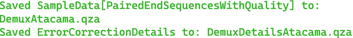
A 2-line text. 1. Saved sample data, Paired End sequences with quality, to Demux Atacama dot q z a. 2. Saved error correction details to, Demux Details Atacama dot q z a.
4.3.5 Summarize the Demultiplexing Results and Examine Quality of the Reads
After demultiplexing, we can use the following commands to create a visualization.

A text reads, Saved Visualization to, Demux Atacama dot q z v.
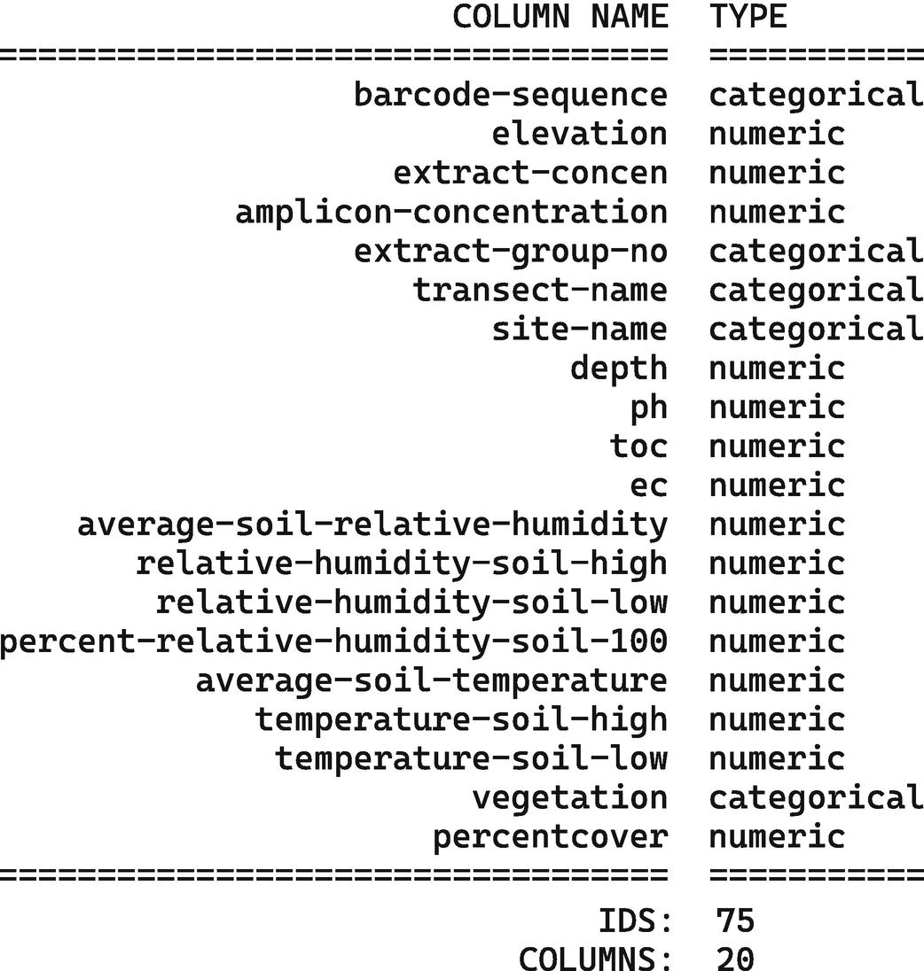
A table of two columns of headers column name and type. Type includes categorical and numeric. The text below the table reads, I D S, 75. Columns, 20.
Inspection of sample metadata for the Atacama soil microbiome study
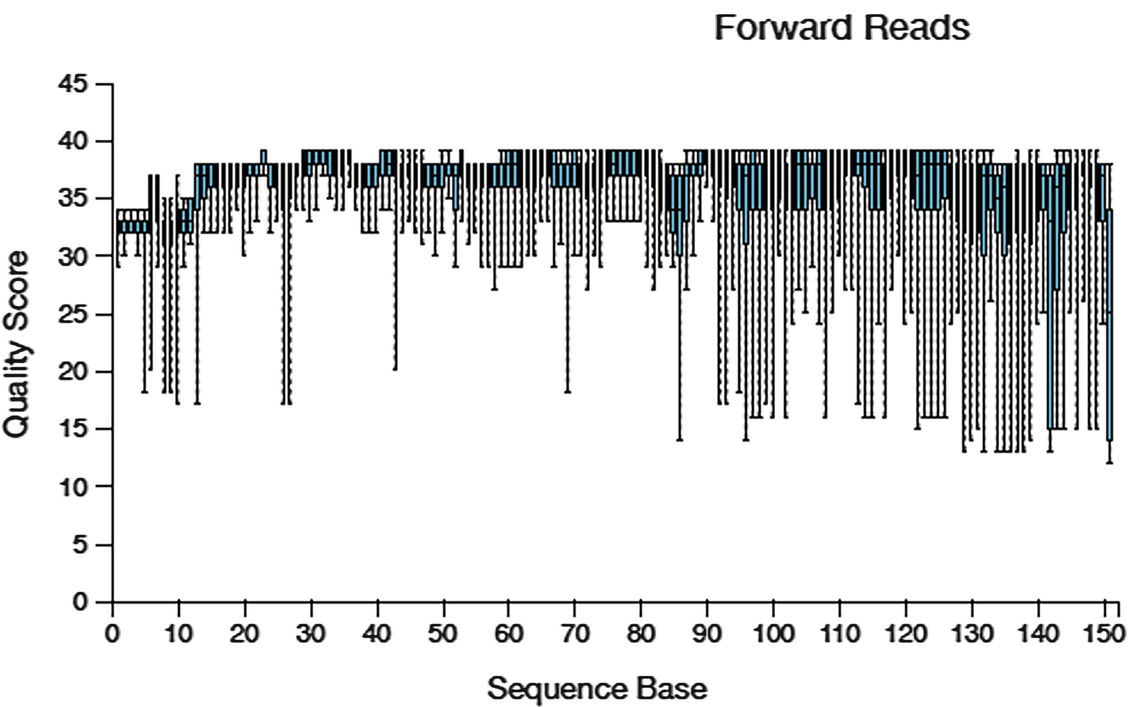
A boxplot of quality score versus sequence base The title is forward reads. The value of the sequencing data ranges between 10 and 40 quality scores. The values are approximated.
Quality score box plots sampled from 10,000 random forward reads for Atcama soil study
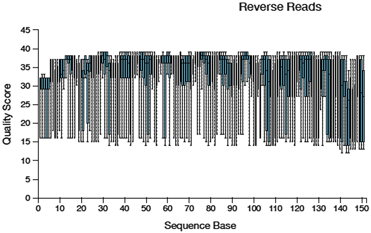
A boxplot of quality score versus sequence base The title is reverse reads. The sequencing data displays a fluctuating trend between 10 and 40 quality scores. The values are approximated.
Quality score box plots sampled from 10,000 random reverse reads for Atcama soil study
4.4 Analyzing Demultiplexed Paired-End FASTQ Data Using Deblur and q2-deblur Plugin
In mouse gut microbiome example (Example 4.1), we show how to conduct denoising and QC filtering sequences to generate feature table and feature data using DADA2 method. Here, we illustrate the Deblur, another denoising method currently available in QIIME 2.
4.4.1 Introduction to Deblur and q2-deblur Plugin
Deblur (Amir et al. 2017) was developed by taking a sub-operational-taxonomic-unit (sub-OTU or sOTU) approach, aiming to identify exact sequences, i.e., obtain putative error-free sequences or single-nucleotide resolution in amplicon studies such as from Illumina MiSeq and HiSeq sequencing platforms. To obtain single-nucleotide resolution, Deblur employs a sample-by-sample approach combined with a greedy algorithm, which compares sequence-to-sequence Hamming distances within a sample to an upper-bound error profile (Amir et al. 2017). Deblur uses an upper error rate bound and a constant probability of indels and the mean read error rate together, this algorithm enabling removing predicted error-derived reads from neighboring sequences when the sequences are aligned together into “sub-OTUs” (Amir et al. 2017). Like ASVs, the sub-OTUs are considered representing the true biological sequences present in the data. The benefits of employing a sample-by-sample approach are that Deblur reduces both memory requirements and computational demand (Amir et al. 2017; Nearing et al. 2018). For the details on algorithm and the development of Deblur, the reader is referred to Sect. 8.3.2.6.
4.4.2 Process Initial Quality Filtering
To obtain high-quality sequence variant data, Deblur uses sequence error profiles to relate erroneous sequence reads to the true biological sequence from which they belong to. To achieve this goal, an initial quality filtering approach should be taken based on quality scores, which was recommended by Bokulich et al. in 2013 (Bokulich et al. 2013). To perform sequence quality control, QIIME 2 has wrapped Deblur quality filtering method in the q2-deblur plugin as implemented in q2-quality-filter.
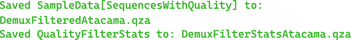
A 2-line text. 1. Saved sample data, sequences with quality, to demux filtered Atacama dot q z a. 2. Saved quality filter stats to demux filter stats Atacama dot q z a.
4.4.3 Preliminary Works for Denoising with Deblur
Step 1: Join reads.
Deblur needs the paired-end sequences jointed before using it to denoise sequences. Because the paired-end sequences have not been jointed, we here join the paired-end reads in QIIME 2 using the q2-vsearch plugin.

A text reads, Saved sample data, joined sequences with quality, to demux joined Atacama dot q z a.
Step 2: Generate a summary of the joined data (in this case, DemuxJoinedAtacama.qza).

A text reads, Saved Visualization to, Demux Joined Atacama dot q z v.
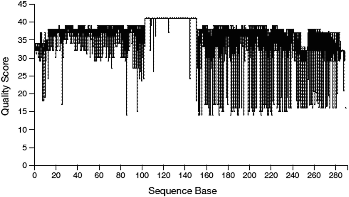
A boxplot of quality score versus sequence base. The sequencing data illustrates a fluctuating trend. The reads have a quality score between 10 and 40. The values are approximated.
Quality score box plots sampled from 10,000 random reads for Atcama soil study
Step 3: Conduct sequence quality control to the sequences using quality-filter q-score-joined
The quality-filter q-score-joined method is identical to quality-filter q-score, except that it operated on joined reads.

A 2-line text. 1. Saved sample data, joined sequences with quality, to demux joined filtered Atacama dot q z a. 2. Saved quality filter stats to demux joined filter stats Atacama dot q z a.
4.4.4 Denoise Sequences with Deblur to Construct Feature Table and Feature Data
The two denoise-sequences methods in the deblur plugin, denoise-16S and denoise-other, are used in different ways. When using denoise-16S, an initial positive filtering step will be performed to discard those reads that have less than 60% identity similarity to sequences from the 85% OTU GreenGenes database. Otherwise Deblur recommends using the denoise-other method. For example, when you apply Deblur to 18S data, you need to specify a reference composed of 18S sequences so that you can filter out sequences which do not appear to be 18S.
The qiime deblur denoise-16S performs sequence quality control for Illumina data using a 16S reference as a positive filter. Currently QIIME 2 only supports forward reads and uses the 88% OTUs from Greengenes 13_8 as the specific reference. Thus, this method is only limited to be used for a 16S amplicon protocol on an Illumina platform.
Deblur can start here to denoise the sequences, which will provide us additional quality control and similarly much higher-quality results as DADA2 did. The crucial action here is to specify a sequence length value for --p-trim-length parameter based on reviewing quality score plots (250 in this case). All the sequences will be trimmed to this length, and any sequences which are not at least this long will be discarded.
Here we use the denoise-16S method. In the following commands, the required inputs (demultiplexed sequences) are one of artifacts: (1) SampleData[SequencesWithQuality], (2) SampleData[PairedEndSequencesWithQuality], or (3) SampleData[JoinedSequencesWithQuality](DemuxJoinedFilteredAtacama.qza), which will be denoised. The parameter --p-trim-length is used to specify sequence trim length, which is also required. Specifying −1 to disable trimming.
The parameters --p-sample-stats or --p-no-sample-stats are used to gather or not gather stats per sample. The default is false. Here we want to gather the stats.
Three outputs need to be required, including --o-table, an artifact of FeatureTable[Frequency], which is the resulting denoised feature table; --o-representative-sequences, an artifact of FeatureData[Sequence], which is the resulting feature sequences; and --o-stats, an artifact of per-sample stats.
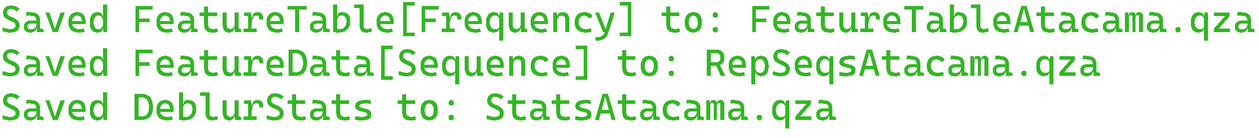
A 3-line text. 1. Saved Feature Table, Frequency, to Feature Table Atacama dot q z a. 2. Saved Feature Data, Sequence, to R e p S e q s Atacama dot q z a. 3. Saved Deblur Stats to Stats Atacama dot q z a.
In above commands, we did not specify other parameters, instead used the defaults: (1) --p-left-trim-len with range(0, None) is used to trim sequence from the 5′ end. The default value of 0 will disable this trim. (2) --p-mean-error is used to specify the mean per nucleotide error for original sequence estimate. The default value is 0.005. (3) --p-indel-prob is used to specify the insertion/deletion (indel) probability (same for N indels). The default value is 0.01. (4) --p-indel-max is used to specify the maximum number of insertion/deletions. The default value is 3. (5) --p-min-reads is used to specify to retain only features appearing at least min-reads across all samples in the resulting feature table. The default value is 10. (6) --p-min-size is used to specify to discard all features with an abundance less than min-size in each sample. The default value is 2. (7) --p-jobs-to-start is used to specify the number of jobs to start (if to run in parallel). The default value is 1. And (8) --p-hashed-feature-ids / --p-no-hashed-feature-ids is used to specify whether or not hash the feature IDs. The default is true.
4.4.5 Summarize the Feature Table and Feature Data from Deblur
As in DADA2 approach, now we can summarize the feature table and feature data and review them via the QIIME2 viewer.

A text reads, Saved Visualization to, Feature Table Atacama dot q z v.

A text reads, Saved Visualization to, R e p S e q s Atacama dot q z v.

A text reads, Saved Visualization to, Demux Joined Filter Stats Atacama dot q z v.
4.4.6 Remarks on DADA2 and Deblur
Both DADA2 and Deblur bioinformatic sequence denoising approaches were proposed to correct sequencing errors to improve taxonomic resolution. Similar to traditional OTU method, both pipelines are self-contained, performing 16S rRNA gene sequencing data from raw sequences (i.e., FASTQ). However, both methods have advanced the sequencing from traditionally binning sequences into 97% OTUs to effectively using the sequences themselves as the unique identifier for a taxon (also referred to 100% OTU).
Both methods perform quality filtering, denoising, and chimera removal and require little data preparation, and don’t need to perform any quality screening prior to running them.
Both DADA2 and Deblur methods have their own advantages and disadvantages. They also share some common properties such as obtaining single-nucleotide resolution. However, we have no intention to compare DADA2 and Deblur methods.
Deblur runs its denoising process sample-by-sample, which helps lower Deblur’s computational requirements; however, it also reduces its ability to correct multi-run.
Another major difference between Deblur and DADA2 is that the built-in Deblur function in QIIME 2 uses a positive filter. That is, they use different strategies to handle errors: DADA2 corrects/changes errors or “erroneous” sequences to match the sequence from which they’re inferred to have arisen. In contrast, Deblur removes those error sequences. By using the default setting Deblur discards reads that do not reach the threshold to any sequence in the 88% representative sequences Greengenes database, which results in the remaining total numbers of sequences and features after denoising using Deblur are less than the total numbers of sequences and features after denoising using DADA2.
Deblur is able to handle processed data whereas DADA2 can only handle raw data. This difference highlights its importance of Deblur because many publicly available datasets are already processed.
Deblur was evaluated having poor performance than DADA2 and open-reference OTU clustering to detect low abundant taxa in the extreme dataset at 97% identity (Nearing et al. 2018).
However, our main goal here is to illustrate these two methods via QIIME 2 and introduce their theories accordingly as necessary to better understand their approaches.
4.5 Summary
In this chapter, we described two methods of building feature table and feature representative sequences data from raw reads, DADA2 and Deblur, illustrated their use in QIIME 2 plugins using two real 16S rRNA microbiome datasets. First, we introduced some general procedures to analyze demultiplexed paired-end FASTQ data including preparation of sample metadata and raw sequence data, importation of data files as Qiime Zipped Artifacts (.qza), as well as examination and visualization of the qualities of the sequence reads. Second, we introduced DADA2 and q2-dada2 plugin and illustrated how to use them to analyze demultiplexed paired-end FASTQ data and specifically to denoise sequences to construct feature table and feature data with q2-dada2 plugin as well as how to summarize the feature table and feature data from q2-dada2 plugin. Third, we illustrated how to analyze multiplexed paired-end FASTQ data using q2-dada2 plugin. Fourth, we introduced Deblur and q2-deblur plugin and illustrated how to use them to analyze demultiplexed paired-end FASTQ Data such as processing initial quality filtering, conducting preliminary works for denoising with Deblur, and particularly denoising sequences with Deblur to construct feature table and feature data and summarize them. Chapter 5 will introduce how to assign taxonomy and build phylogenetic tree. Chapter 6 will introduce the traditional OTUs clustering methods.